To create an FPP model from CAD model you need to follow a top-down procedure. This top-down process is mostly incorporated in the model explorer of Artist Studio.
The whole procedure is divided into two parts of Artist Studio which are Patch Artist and Motion Artist. We will start with Patch Artist, which provides various modules for fiber placement.
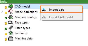
Import the model as explained previously in “Getting started” section. Alternatively, the user can also import CAD model by clicking right on CADmodel and then select Importpart.
Artist Studio supports these formats of 3D model:
Brep Files
Iges Files
Step Files
Stl Files
After importing the CAD model you can use various tools of Ribbon bar such as changing orientation, viewing in different viewports, changing render mode and render style.
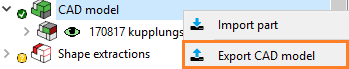
Once the CAD model is imported in Artist Studio, the user can export the CAD model at any stage of FPP process to reconstruct or remodel using any other external software. To export the CAD model you can click right on CADmodel and then select ExportCADmodel.
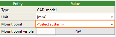
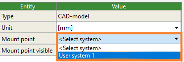
The mount point is a position on the CAD model that defines the center of the robot to tool mount.
It is defined as the position on the tool that corresponds to the center point of the tool mounting, i.e. the center of
the mounting plate on the tool’s surface.
Hint
For easier selection, it is generally recommended to use the mount point as zero coordinate value in your CAD model.
It can be selected after selecting the CAD Model root item in the tree:
Choose a coordinate system that has been defined in your CAD model in the drop-down list:
Depending on the imported CAD file, the list might be empty. In this case, please define a coordinate system
as explained in detail in Create system.
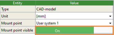
The created Mount point can be displayed in Patch Artist as well as Motion Artist by setting
it to visible:
This functionality is only applicable to SAMBA Step systems.
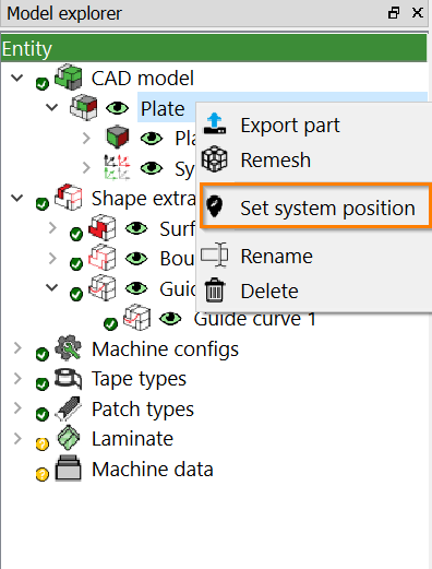
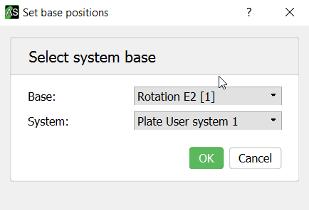
With the Setsystemposition functionality, it is possible to automatically align systems in the CAD model
with pre-defined positions of a machine. Based on the selected position (Base) and the CAD model system (System),
the appropriate mount point system is calculated and set.
Click right on the imported CAD model and select the Setsystemposition option.
A pop-up dialog will open:
Select the Base from the dropdown. On SAMBA Step machines the Mount frame has to be set to the values of a measured base of the machine.
This can then be selected in the drop-down.
Select the corresponding CAD model system as System
Click OK button to confirm.
Once OK has been clicked, Artist Studio will calculate the correct mount system
and set it as the active mount point.
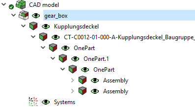
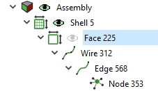
A complete model layout from the model to assemblies, assembly to solids, solid to shells, shell to faces, face to wires and so on can be viewed in Artist Studio.
To view parts or subparts of the 3D model just click on the drop-down button as shown below:
It is also possible to import coordinate systems together with the CAD data which will be shown by Systems in the layout.
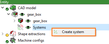
The CAD models can be specified with their own coordinate systems (local) which will be translated according to the global coordinate system of Artist Studio. A user system can also be used as the tool’s Mount point or to define the fiber orientation. To create a system, expand the layout of the CAD model by clicking on the drop-down button.
Right click on the Systems button and click on Createsystem.
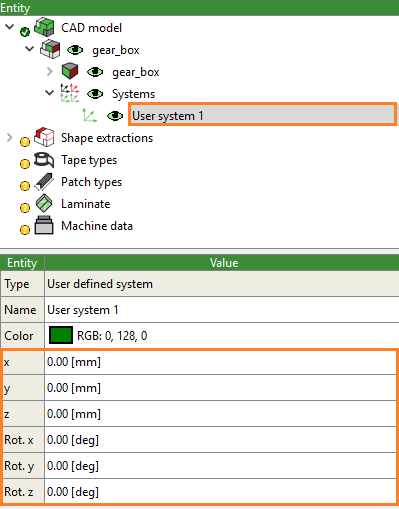
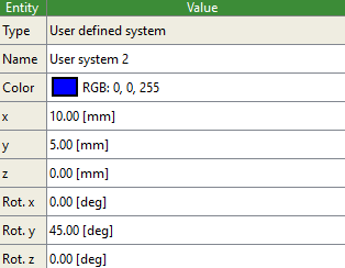
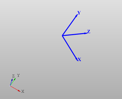
This will create a system where the user can define the coordinate system for the CAD model in its Property editor window.
Enter here the values for xyz coordinate system and choose the color depending on the requirements.
Following user defined coordinate system will be created.
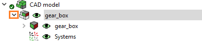
The eye button provides the functionality to show or hide parts of the model. To hide any part just click on the green eye and click on the colorless eye to view parts.
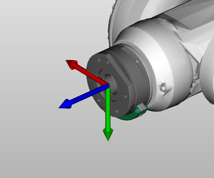
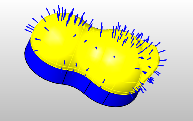
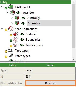
Every CAD model has normals. Normals influence the direction from where Picker places the layup. The orientation of the normals should be pointing outside the geometry for ideal placement of the Laminate.
Viewing normals
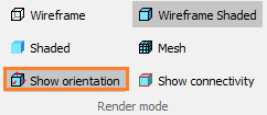
The easiest way to check normals is to select on Showorientation from the ribbon bar under Rendermode group.
And then select a face or shell from the CAD model.
Reversing normals
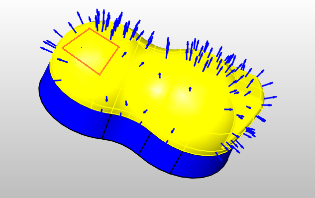
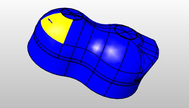
Sometimes, there is a need to reverse the normals for generating layup of the FPP model. As shown in the image below, the orientation of the marked face is pointing inside.
For flipping the normal, select the face from the CAD model for which you want to reverse the orientation of the normal. You can also select a shell to reverse the orientation of all the faces consisted in the shell. Now, click on the Reverse button from the property window.
The normal of the selected face will be reversed as shown below:
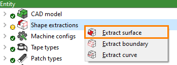
After checking the normals, the next step to create FPP model is to extract shapes such as Surface, Boundaries, Master Curves and Points. Click on the drop-down button to define them. Shape extraction is incorporated with Selection tools for easy and multiple selections of faces or curves. Click here to know more about them in details.
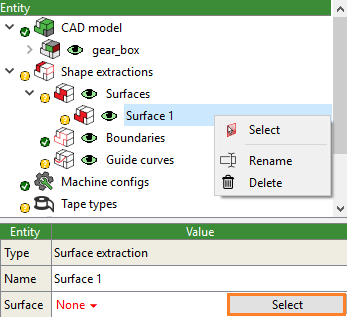
The surface is a CAD-based entity that describes the part surface on which a layup would be generated. Right click on Shapeextractions and click on Extractsurface to extract surfaces.
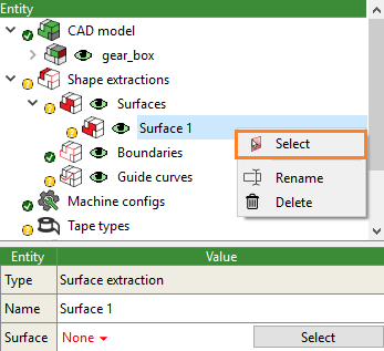
This will create an empty surface where you can extract surface from the CAD model. Surfaces can be selected in two ways:
From entity window: Right click on the empty surface and click on the Select option.
From property window: Select the created surface and click on the Select button from Property window.
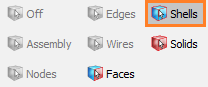
On clicking either of the Select button, selection toolbox will appear. Use the toolbox to extract the surfaces. Before extracting the surface, select Pickingtype from the Ribbon bar.
This can be done in 3 ways:
Manual Selection - Select the face by normal clicking on the face. For multi-selection, select the faces with the Shift key pressed.
- Select one face and click on this icon. With every click, adjacent faces will be selected.
- Select one face of the assembly and then click on this icon. It will select the whole assembly corresponding to the selected face.
Next step after selecting a surface is to click on the green tick as shown below.
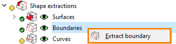
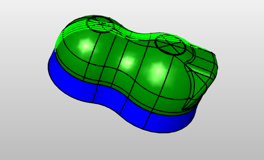
The CAD model must at least contain a boundary line enclosing the area which is supposed to be filled with layup. This is the so-called patch boundary.
The patch boundary defines the area where the patch would be placed by the manufacturing cell. However, it is not necessary to explicitly define a boundary. Patch Artist automatically extracts the boundary of a surface as a Boundary. To explicitly extract a boundary follow these steps:
Click right on Boundaries under Shape extraction and then click on Extractboundary.
With the creation of boundaries, you can define areal constraints for your layup. For creating a boundary just click on the selected surface which will create a node on a surface. Whenever you make a new point by clicking on the surface, Artist Studio will join the previous point with the new one. You should make sure that the created boundary is enclosing the surface.
Using the button Select from the Property window allows easy extraction of boundaries:
Here, you can create a boundary by simply selecting the edges of the surface depending upon the requirements.
At first, select the Pickingtype from the Ribbon bar either edges or wires.
This can be done in 3 ways:
Manual Selection - Select the edge by clicking on the edge. For multi-selection select the edges with the Shift key pressed.
- Select one edge and click on this icon. With every click, the adjacent edges will be selected.
- Select one edge of the assembly and click on this icon. It will select the whole assembly corresponding to the selected surface.
Next step after selecting a boundary is to click on the green tick as shown below.
tip - Keep the Control key pressed for selecting more than one edge.
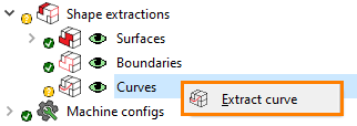
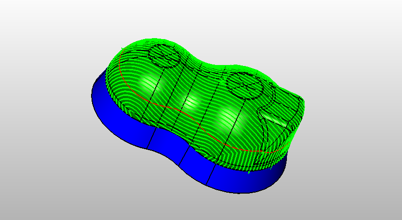
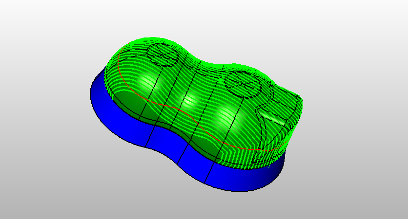
The orientation of the patches inside a layer is in most cases defined by a so called Master curve. One way of creating such a Master curve is by extracting a Curve from a CAD part. Follow these steps to create a Curve:
Click right on Curves under Shape extractions and then click on Extractcurve.
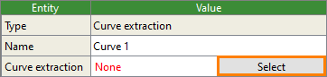
To extract a Curve the option Select is used: Simply click on the edges or wires for extraction of a Curve in the same fashion as explained above for the boundary extraction.
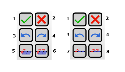
Selection toolbox in viewport
Selection toolbox contains tools for selecting different shapes such as surfaces, boundaries and curves. Various selection tools are shown below:
For saving the selection.
To close the selection toolbox.
Undo
Redo
Select adjacent surfaces - First select a face. Then with every click on this tool, adjacent faces will be selected from the model.
Select all connecting surfaces - This gives user more power. With one click, all faces corresponding to the selected face in one assembly will be selected.
Select adjacent edges - Here, first select an edge. Adjacent edges (making the angle less than or equal to 15°) will be selected with every click on this tool.
Select all connecting edges - Select an edge from the assembly. With one click on this button, all edges (making the angle less than or equal to 15°) will be selected.
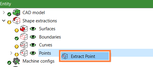
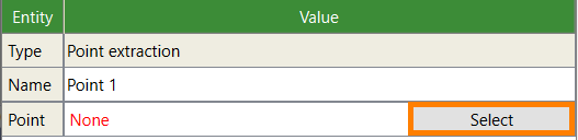
Some methods for defining a Master curve depend on a point extraction. Follow these steps to create a Point:
Click right on Points under Shape extractions and then click on Extractpoint.
To extract an existing node the option Select is used: any CAD node can be picked.
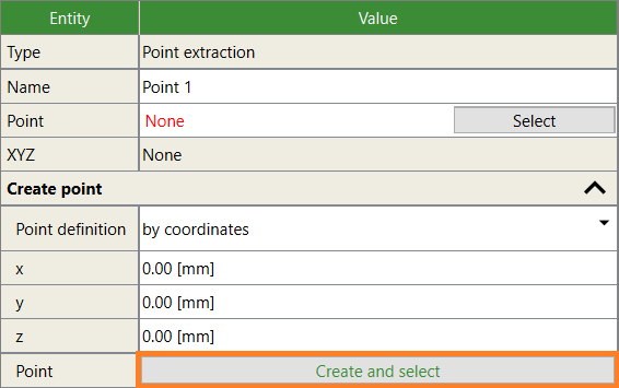
To create a new point the option Createandselect is used.
This can be done in 3 ways:
by coordinates - Creates a point with given x, y and z coordinates.
from curve - Select a curve extraction, a system, a system axis and an extremum type. Artist Studio will find the first point on the curve that is either closest to or furthest away from the plane defined by the system and the selected axis.
from surface - Select a surface extraction, a system, a system axis and an extremum type. Artist Studio will find the first point on the surface that is either closest to or furthest away from the plane defined by the system and the selected axis.
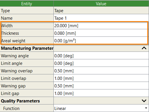
Within this option, the user can define Width, Thickness and Areal weight of the tape. These are important for fiber layup placement on the model and these parameters will define the quality of the output. Moreover, Areal weight is required to calculate the weight of the fiber material in the Laminate.
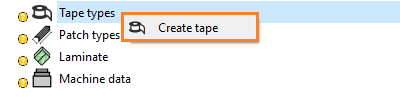
Click right on Tapetypes then click on Createtape.
After clicking on Createtape, enter the values for Width, Thickness and Arealweight of the specific tape.
Note
All the other values will be automatically imported when loading a CATIA file.
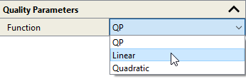
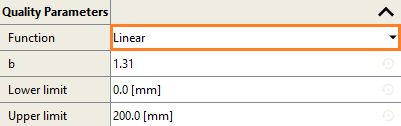
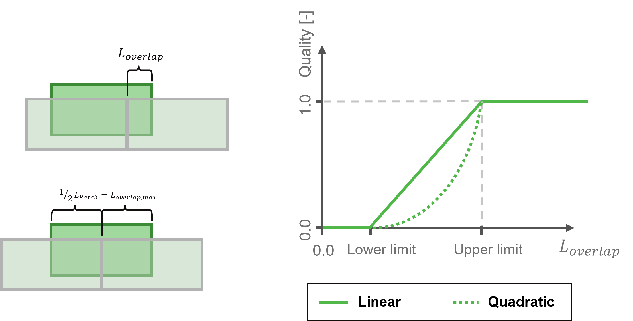
The user can make changes to the quality criterion of a tape which is used for layup overlap optimization. This option provides three types of quality functions: QP, Linear and Quadratic. All functions will favor higher overlaps between patches during optimization. However, their convergence behavior is vastly different. When in doubt use the Quadratic approach.
QP - A complex physical strength based quality criterion derived from Cevotec’s research on optimal FPP layups. Only valid for Cevotec dry fiber material.
Linear - Linear interpolation between a lower and an upper limit. Overlap lengths below the defined lower limit will have the quality value of 0.0, while those above the upper limit will get the the maximum quality 1.0 assigned. Please refer to Fig. 6.1 for details. The factor b specifies the drop-off of the influence of a gap in the direction of Thickness and usually doesn’t need to be modified by the user. The Linear option is only recommended in combination with layers with two sublayers. For more sublayers please use Quadratic.
Quadratic - Similar settings as Linear but with a quadratic interpolation between lower and upper limit. Best suited for layers with more than two sublayers. See Fig. 6.1 for a comparison with the Linear quality function.
Fig. 6.1 Linear and Quadratic quality criterion as a function of patch overlap length
Note
The maximum overlap length between two patches is always half the patch length. This doesn’t mean, though, that the upper limit can’t be higher (but you will never be able to achieve an overall laminate quality of ~ 1.0). See also Fig. 6.1.
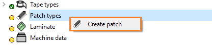
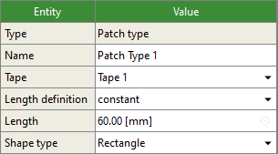
To create a new patch type, right-click on Patchtypes in the tree and select CreatePatch. A new patch type will be added,
and its properties can be configured via the property window:
Name
The name of the patch type.
Tape
Specifies the type of tape used. Choose a tape type from the drop-down menu.
Length definition
Specifies how the length of patches in this type is defined. Select one of the following options from the drop-down menu:
constant
All patches in this type will have the same fixed length, defined by the Length property.
continuous
Patch lengths vary within a defined range (minimum and maximum). Patches can take any length within this range.
Note
The continuous option may result in a large number of unique patch shapes, which can negatively impact
production speed and yield. It is recommended for experimental or exploratory use only.
Note
Continuous lengths do not work reliably on closed curves.
discrete
Patch lengths vary within a predefined set of discrete values. Only the specified lengths will be used (e.g.,
40 mm, 60 mm, 80 mm, 92 mm).
For more information on automatic variable (continuous/discrete) patch length and its use see Automatic variable patch length.
Length
Defines the actual length values based on the selected Lengthdefinition:
constant
A single value. All patches have this exact length.
continuous
Two separate values: Min.length and Max.length. Patches can have any length between these two values.
discrete
A list of allowed patch lengths, given as a comma-separated list in [mm].
Shape type
Specifies the geometry of the patch’s cutting edges. Options depend on the capabilities of your manufacturing system:
Rectangle
A standard rectangular patch with no additional shape parameters.
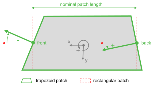
Trapezoid
A trapezoidal patch with configurable front and back angles.
Trapezoids must first be enabled in the root item of the patch types.
The angles are defined relative to the patch’s x-axis, using the right-hand rule with respect to the patch normal.
A 0° angle corresponds to a rectangular edge. The nominal patch length is measured along the centerline.
A trapezoid can degenerate into a triangle if a short patch length and large opposing angles are used.
Isosceles trapezoid
Similar to Trapezoid, but the front and back angles are coupled.
You set only the front angle; the back angle is automatically set to the same magnitude with the opposite sign.
Note
Trapezoid shapes can be used for laminate creation and FEA. However, not all production systems
can manufacture non-rectangular patches.
Machine configurations in Artist Studio contain essential data about your
production system, and are stored within the “Machine Configs” part of FPP
files. This data includes Motion Artist defaults specific to each system.
While machine configurations are primarily used in Motion Artist to ensure
precise robot movement generation, some configuration details also impact
laminate design in Patch Artist. For example, estimating the cutting scrap
rate depends on the length of a fixed gap between patches, which is needed
whenever the trapezoidal angle changes.
If your main focus is laminate design in Patch Artist, creating machine
configurations can initially be optional. They only need to be completed
before generating machine data in Motion Artist.
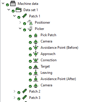
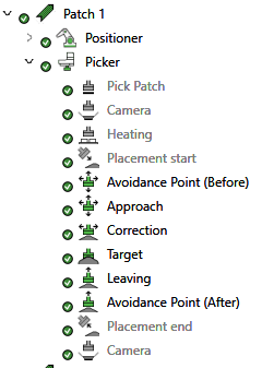
The picker follows a series of positions during operation, usually pick, camera,
heating, placement start, approach, correction, target, rolling, extra leaving/approach,
contact, leaving, placement end, and a final camera check. Which of these movements
are actually used depends on the SAMBA system type.
Movements responsible for deposition of a patch (i.e., from approach to leaving)
are generated by Motion Artist and exported in the final robot program. For more
details, see Patching section. Users can
add additional avoidance, approach or leaving movements, which also become a part
of the robot program. In contrast, initial and final positions - like pick,
camera, heating, and placement start/end (gray in the screenshot above) - are
manually taught during system setup and only simulated in Motion Artist, but
typically not exported.
To ensure that Motion Artist simulations align with real-world operations, and thus
to enable effective collision detection and avoidance, these exact taught positions
should be provided to Artist Studio as JSON files (in the ‘rob’ subfolder of the
Artist Studio installation, or if needed in a custom folder, see
Custom cells).
Note
For SAMBA Pro and SAMBA Step M, the heating position is not taught, and it is
exported in robot programs. Its initial default value is still loaded from a
JSON file.
These files are usually initially provided by Cevotec after Factory Acceptance Testing
(FAT). If any positions are retaught or modified, users should update these JSON files
and share them among engineers using Artist Studio. Once loaded in the Machine Configs
section in Artist Studio, these default values can be adjusted as needed.
For systems with two robots, the machine configuration includes a default deposition
frame, which can either be determined within the production system or manually set
in Motion Artist. Note that deposit optimization may adjust this default position
per patch.
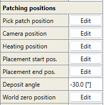
The following taught positions are primarily used for simulation and collision
detection and are generally not included in the robot program:
pickPatchPosition: Pickup position on the conveyor belt.
cameraPosition: Position above the camera, used before and, if needed, after
deposition.
auxiliaryPosition: Position after the camera to which the robot can move even
while waiting for the vision to compute.
heatingPosition: Position above the heating unit.
placementStartPosition: Last taught position the picker reaches
before deposition (for systems made in 2024 or later).
placementEndPosition: First taught position the picker reaches
after deposition (for systems made in 2024 or later).
Special positions for systems with two robots:
depositFrame: Default point of contact between the picker gripper and
the positioner tool during patch placement.
worldZeroPosition: Reference position for exporting picker movements,
usually matching the picker robot’s coordinate system. Taught positions are
represented relative to this position.
Special positions for systems with a rotational axis positioner:
depositAngle: Default angle of the point of contact between the picker
gripper and the positioner tool during patch placement. The deposition
point’s distance from the axis depends on the tool’s shape after rotation.
Push-in direction is defined relative to the tool surface’s normal at
this deposition point, with optional manual adjustments.
Special positions for systems with one robot:
coordinateRootPosition: Fixed offset of the picker’s root position.
worldZeroPosition: Reference point (relative to the coordinate root)
for export of picker movements, often a designated table corner in 2D placement.
Taught positions are represented relative to this position.
mountFrame: Used for calculating mount points via
the “Set System Position” dialog, see Set system position.
depositExternalAxes: Contains the default values of the external axes
of the picker robot to use during deposition.
Machine config positions are represented in one of 4 formats:
Transformation: Defines a position with a translation and rotation.
Positions that are represented in this format: coordinate root, world zero, deposit frame, mount frame.
Example JSON:
Angle: Defines a position with a single angle in degrees.
Positions that are represented in this format: deposit angle.
Example JSON:
"depositAngle":-35.0
External axes: Defines a position with a value for each external axis of a robot.
Currently the only system with a robot that has external axes is Samba Step L (1 external linear axis).
Positions that are represented in this format: deposit external axes.
Example JSON:
"depositExternalAxes":[-400.0,0.0,55.3]
Taught position: Defines a taught position with a transformation, external axis values and status/turn values (for KUKA robots).
Positions that are represented in this format: pick patch, camera, heating, auxiliary, placement start, placement end.
Example JSON:
Target speed: A value between 0 and 100% to adjust the speed of the
gripper as it moves to the Target position. Lower speeds
may improve the uniform draping of the patch on the surface.
Target acceleration: A value between 0 and 100% to adjust the
deceleration of the gripper in the final part of the movement to the Target position.
Touch time: The wait time of the gripper at the Target (pushed-in) position.
Blow off delay: The time interval between the gripper reaching the Target (pushed-in)
position and the initiation of the blow-off process. This delay is always
shorter than the touch time.
Retraction acceleration: A value between 0 and 100% to adjust the
acceleration of the gripper as it moves away from the Target position.
Retraction speed: A value between 0 and 100% to adjust the speed of
the gripper as it moves away from the Target position. Lower speeds may
help prevent patches from being peeled away from highly curved surfaces.
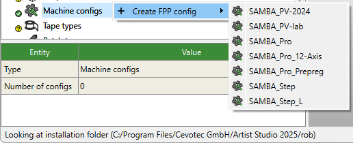
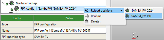
6.5.5. Creating, modifying and resetting machine configurations
Machine configurations are saved in the FPP file.
To create a new machine configuration from a JSON file, right-click on the
“Machine Configs” item in the Artist Studio tree.
Once created, you can edit the positions and values as needed. If necessary,
reset the configuration to values from any JSON file for the same machine type.
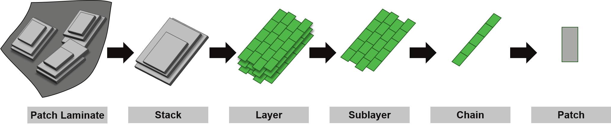
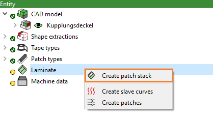
Patch Artist uses a discontinuous patch based approach to build a so-called Patch Laminate. It is the root element in this hierarchical structure. It exists only once in every project and contains all other entities.
As shown in the above figure, Layups are organized hierarchically in containers to reduce complexity. The user can view Number of stacks, layers, sub-layers, chains, patches in the Property editor window.
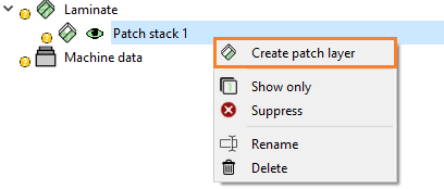
The next (hierarchically) lower level is called Stack. Stack is the first branch of Laminate. The user can create any number of stacks depending on the model under Laminate. Click right on Laminate and then click on Createpatchstack.
Stack is a collection of several (partially) overlapping layers.
Advancing further down the hierarchy, the next lower level after Stack is layers. There can be any number of layers under one Stack. A layer describes a layup of multiple patches that can be defined by common properties. To create a layer, right click on the created stack Patchstack1 and select Createpatchlayer from the context menu.
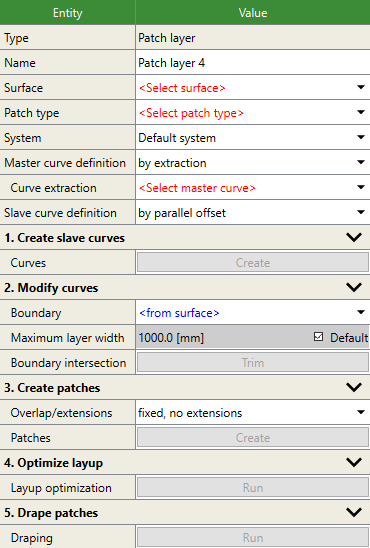
Let us understand the Property window of Patch Layer in detail:
Type
Shows the type of entity selected above by the user. It would be Patch layer in this case.
Name
Shows name of the layer. The user can rename or delete by right-clicking on the layer.
Surface
Select previously extracted surface from the drop-down menu. Note that only one type of surface could be selected under one type of layer.
Patch type
Within this option, the user can select previously created patch types. Only one type of patch can be selected per layer.
System
You can select a previously imported or manually created coordinate system for this layer. If you choose to keep the Default system,
a system similar to the global coordinate system shown in the viewer is used. Be aware that not all methods of master or slave curve creation
require a coordinate system.
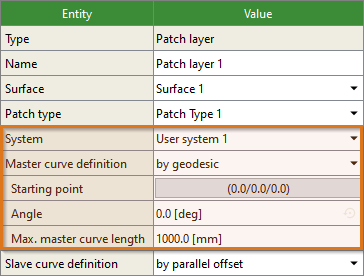
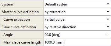
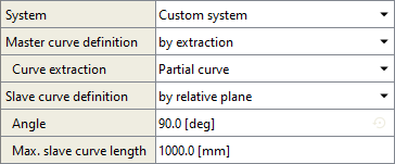
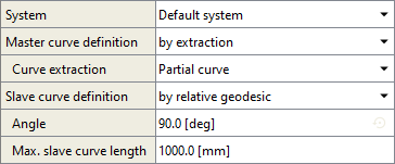
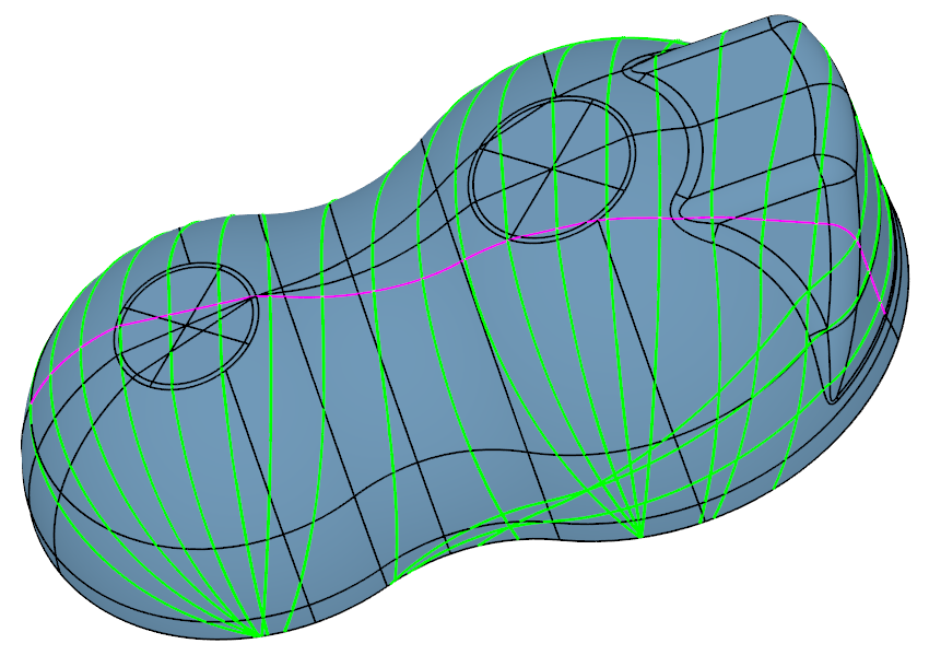
Master curve definition
The Master curve is the reference curve for the creation of Slave curves. There are multiple ways to create a Master curve. See Master curve definition for details.
Slave curve definition
Slave curves define the orientation of the patches to be created. For this purpose, the start and end point of each patch lies (at least initially) on a Slave curve. See Slave curve definition for details.
The master curve either acts by itself as a reference for the desired fiber orientation or it is used to create seed points for a subsequent slave curve generation. We will dive deeper into this topic in the following section on slave curve creation.
Settings relevant to master curve creation are depicted below. Depending on the selected curve definition not all settings will be available.
Master curve definition
Algorithm for the creation of the master curve. See next section for details.
Curve extraction
Selection of an existing curve extraction using a drop-down list. Please refer to Extract curve for guidance on how to create a curve extraction.
System
Some curve creation methods require a reference orientation in form of a vector. The x-axis of a coordinate system provides such a vector. Please refer to Create system for guidance on how to create a system.
Starting point
The starting point for curve creation. Selection of an existing point extraction using a drop-down list. Please refer to Extract point for guidance on how to create a point extraction.
Angle
An angle relative to the projection of the system x-axis onto the local surface plane at the location of the starting point. Defines the curve orientation.
Max. master curve length
The maximum length of the curve, applied in both curve creation directions (i.e. maximum combined length will be 2x this length).
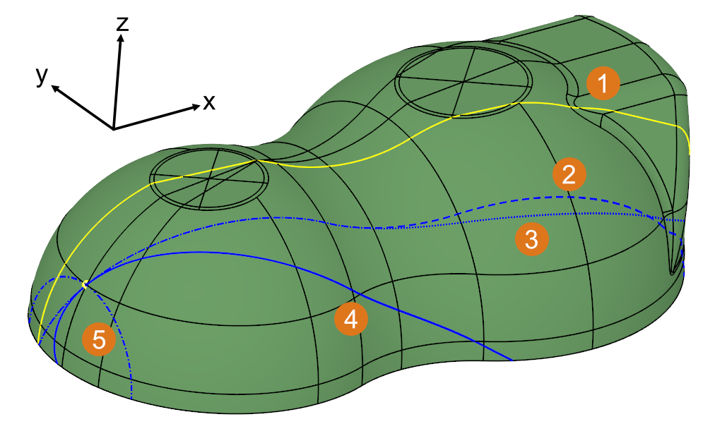
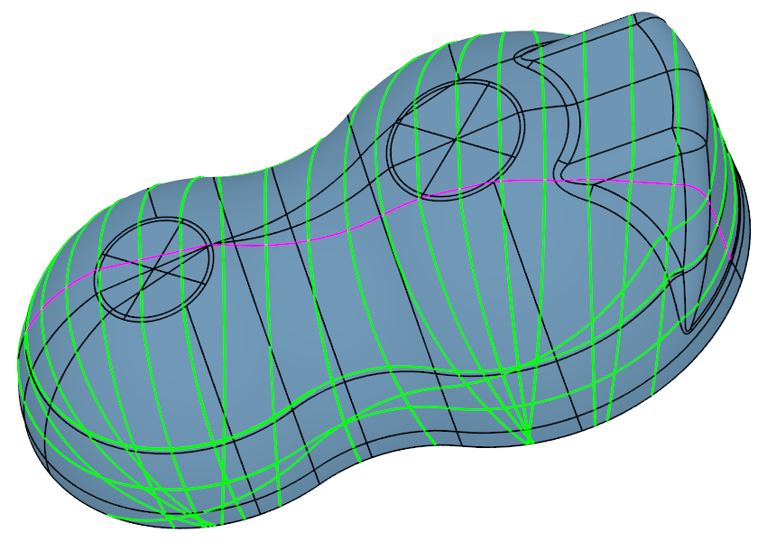
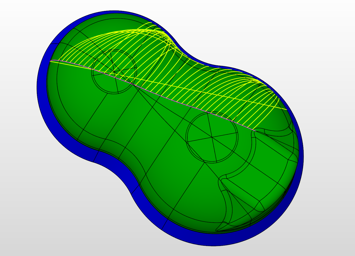
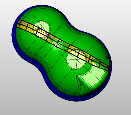
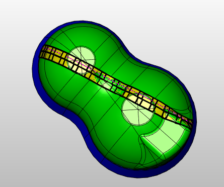
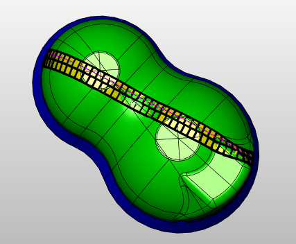
The following figure shows how the curve fiber orientation is calculated by using above settings.
Fig. 6.2 The process of deriving the curve orientation from starting point, system and angle.
There are multiple ways to define your master curve. Select the one that is most suitable for the laminate design task at hand.
Fig. 6.3 Curve creation examples. When supported by the method, an angle of -30° was chosen for the curve.
byextraction
Select an existing Curve extraction from the drop-down menu. There are no additional settings available. Use this method if you want your curve to follow existing edges of your model or if your design requires a complex shaped curve that can only be realized using an external CAD tool.
byplane
The curve will follow the intersection of the surface with the plane normal orthogonal to the local surface plane at the starting point. Only the byplane and byexternalplane curve types can form closed curves.
bygeodesic
The curve will follow the shortest path along the surface. It can also be interpreted as a curve that is free from lateral forces when tension is applied on the curve. It is therefore commonly used in winding applications.
bydirection
The curve will follow this reference orientation by locally projecting the
byexternalplane
Similar to byplane but not affected by the surface normal at the starting point. Intersects the surface with a plane that is normal to the system x-axis and runs through the starting point. Just like byplane, this method is able to form closed curves.
The following table shows an overview of required settings for each algorithm.
Fig. 6.4 Available layer settings based on selected master curve definition
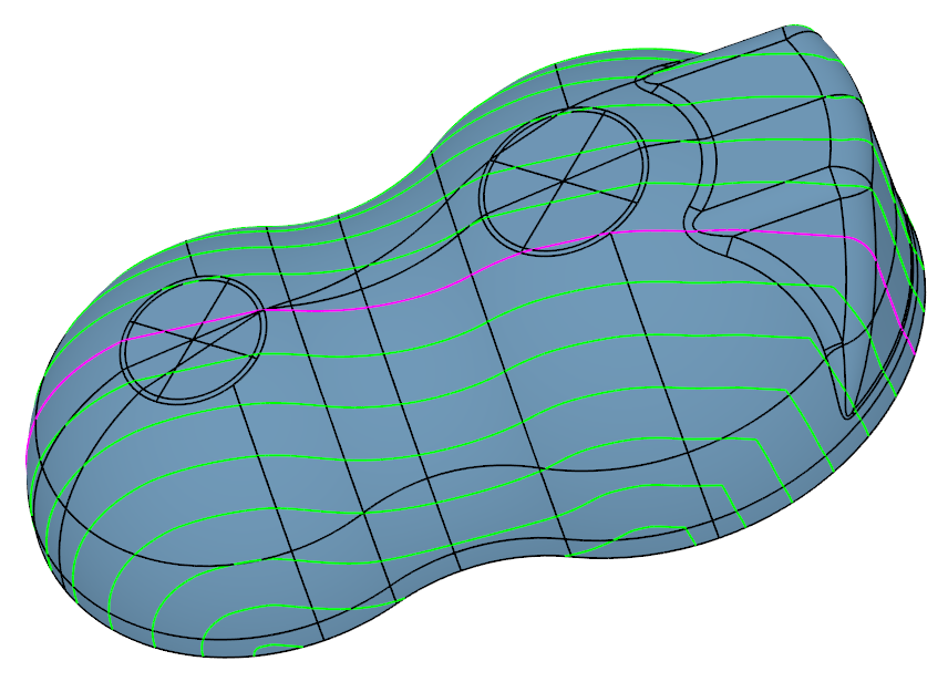
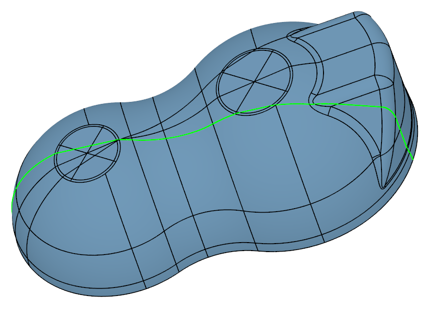
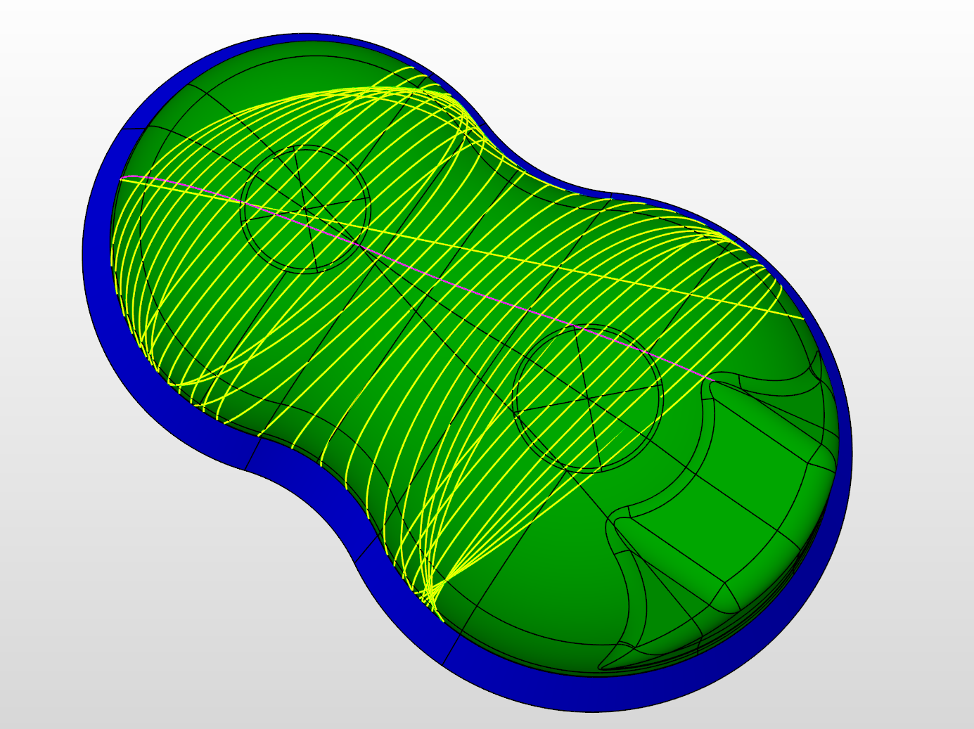
There are multiple methods to create Slave curves that can generally be divided into two groups, based on their usage of the Master curve:
6.6.2.3.1. Master curve as reference for fiber orientation
When selecting byparalleloffset, parallel offset curves are created from the Master curve. The distance between all curves will be equal, resulting in a minimal amount of gaps and overlaps in the laminate. However, in areas of high curvature (curve and/or surface) only patch start and end point are guaranteed to be exactly on the curve (this is the case for all slave curve definitions). The masteronly slave curve definition is a convenience function that covers the special case of the parallel offset, where only a single curve (the master curve) is used.
Note
You will also see the option [BETA]byparalleloffset.
This denotes an experimental version of a new parallel offset algorithm that can handle certain cases better than the default one.
Note that the new algorithm’s speed and accuracy heavily depend on the mesh density of the surface.
Table 6.1 Examples for curve definitions based on master curve as reference for fiber orientation
Seed points are created along the Master curve. For each point, a curve is created with the same algorithm as described for the creation of the Master curve (bydirection, byplane, …). In contrast to the parallel offset, the curves are usually only equidistant along the Master curve. In addition, there is a second group of curve creation algorithms that behaves similarly but uses the local curve tangent of each seed point as reference orientation. Consequently, they are named following a byrelative... scheme.
Warning
As of Artist Studio version 1.3.34, the angle definition of the byrelativeplane slave curve method slightly changed. An angle of 0° used to create a curve that is orthogonal to the master curve. To be in sync with other “relative” methods, this value is now defined to be 90°.
The table below shows examples of all curve creation methods.
Table 6.2 Examples for curve definitions based on seed-points generated from master curve
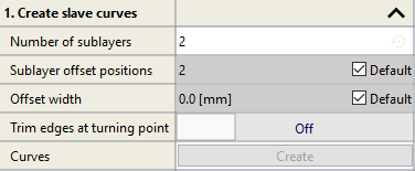
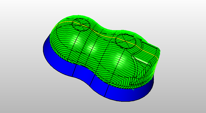
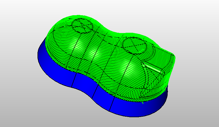
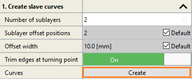
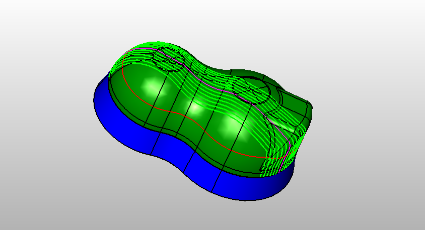
Slave curves are the curves which are created by offsetting the Master curve with a constant offset value in order to cover the Patch zone. Click on the drop-down menu to make changes in the default settings. The user can also create Slave curves from the context menu of the created Patch layer.
Number of sublayers
Enter the Number of sublayers for creating FPP model.
Sublayer offset positions
Each sublayer in a Layer should be also transversally shifted against each other to increase the mechanical performance. The offset position has to be between zero and the patch width. If the number of sublayers is higher than the number of sublayer positions then curve pattern will be repeated after the number of sublayers. The default value of Sublayer offset positions changes with respect to Number of sublayers. To make changes in the default value, uncheck the default button and enter the value for Number of offset positions here.
This option allows the user to enable or disable the propagation of slave curves exclusively in the forward direction, relative to each curve’s starting point (a seed point on the corresponding master curve). It is available only when the selected slave curve definition is one of the methods described in Master curve as base for seed points.
By switching ON or OFF this option, you can observe the following changes in your geometry:
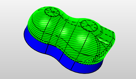
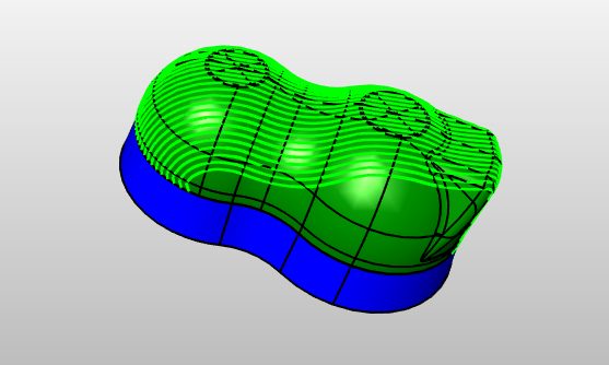
Within this option, the user can switch ON or OFF trimming of edges at the turning point of Master curve. Let’s assume that Master curve is not completely covering the surface. By switching ON or OFF this option, you can observe the following changes in your geometry:
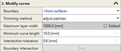
Within this option, the user can modify Slave curves depending on the requirements. Click on the drop-down menu to make changes.
Patch boundary
Select the extracted boundary for defining a patch boundary. By default, Patch Artist takes surface’s boundary to define Patch boundary.
Trimming method
Adjust patches creates intersections and removes all patches that are outside the boundary. Adjust curves trims the curves between the first and the last intersection with the boundary.
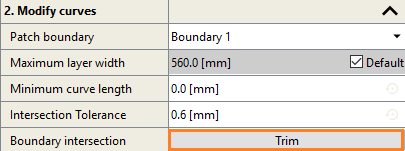
Maximum layer width
By changing Maximum layer width, the user can increase or decrease the area covered by the patches. Its value should be greater than the width of the tape otherwise Patch Artist would not create Slave curves.
Minimum curve length is the value which defines the minimum length of Slave curve. Patch Artist will not create Slave curves whose length is below this value.
It is defined as a tolerance between the intersection of the extracted boundary and Slave curves.
Boundary intersection
This button is only active if the user has selected a patch boundary. However, it is not required to calculate intersections if the boundary is at the edge of the surface.
Click on the Trim button to modify Slave curves.
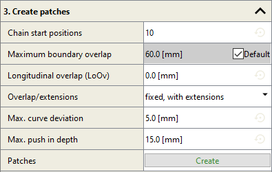
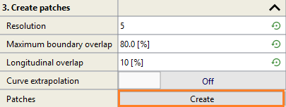
This step will generate patches on the surface based on the Slave curves created above. Click on the drop-down menu to make changes in the default settings. The user can also create Patches from the context menu of the created Patch layer.
Chain start position
Within this option, you can define the number of starting positions for chains.
It is recommended to use 10 (default value) as Chain start position for a good quality of layup but for fast optimization and where quality doesn’t matter you can decrease this value.
Maximum boundary overlap
It defines the allowable overlap between the patch and patch boundary.
The user should enter a small value of Maximum boundary overlap to reduce scrap but small values may result into large gaps close to patch boundaries.
An appropriate value for Maximum boundary overlap should be entered depending on the requirements. To generate patches outside the boundary,
the user should define Curve extrapolation length for creating Slave curves outside the extracted boundary.
Let’s take 60 mm as Curve extrapolation length for the example shown below. For better understanding, the bottom assembly of Gear box is hidden.
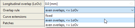
By default the Longitudinal overlap specified above is used as a fixed value, which will generally result in a gap between the end of the chain’s last patch, and the end of the curve.
In order to fully cover a curve exactly from the start to the end, the restrictions on gaps and overlaps can be loosened by having the chosen overlap value act as a lower or upper limit instead.
Note that for open curves with even overlaps, changing the chain start position will not shift the chain.
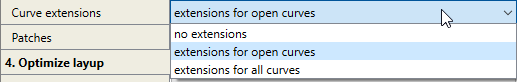
Curve extensions
As described in FPP basics, sometimes there is a need to extrapolate Slave curves. Here, you can decide to extend some or all of the curves.
Max. curve deviation
Note
Only for automatic variable patch length based on curvature
Defines the maximum allowed angular deviation between the patch centerline and the corresponding segment of the guide curve.
To meet this requirement, patches are automatically shortened in regions where the guide curve has high in-plane curvature. This results
in shorter patches on curved segments and longer patches on straighter parts of the curve.
A smaller value enforces closer alignment with the curve.
A value of 90° disables the effect of this setting entirely.
Max. push-in depth
Note
Only for automatic variable patch length based on curvature
Specifies the maximum allowed push-in depth required by the gripper to place a patch on the surface. If this limit is exceeded,
patches will be shortened to reduce the required push-in. This results in shorter patches in areas with higher surface curvature
(non-flat regions). Set this value based on the physical constraints of your gripper.
A value larger than the maximum patch length effectively disables this constraint.
Patches
Click on Create button to generate Patches on the model.
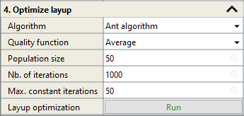
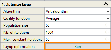
This part of Model tree consists of various options to optimize the layup by making changes in the default settings.
Algorithm
Ant algorithm is an heuristic population based algorithm that uses a number of individuals
(each representing a solution) that interact with each other over the specified number of iterations to find an
optimum solution. However, the user can choose a high value for Nb. of iterations and Population size for a
better solution but it will consume more time.
Quality function
Select the type of quality required for the CAD model such as minimum or average.
Population size
Enter here the number of values you want per iteration for Ant Algorithm.
Nb. of iterations
Within this option, enter the maximum number of iterations required for optimization of layups.
Max constant iterations
Here, enter the number of iterations you want to be performed by the selected algorithm.
It is a stop criterion for optimization which means if the result of the optimization is coming out constant for
the entered number of Max constant iterations then optimization algorithm will stop.
Recommended number of Max constant iterations is between 10 to 50.
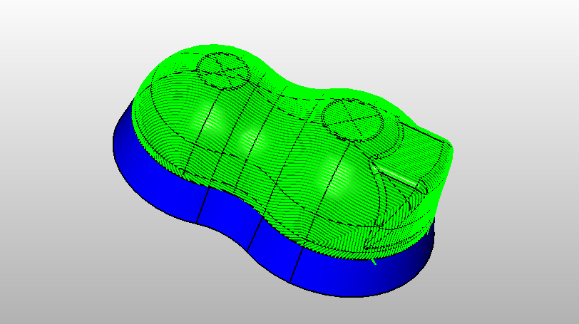
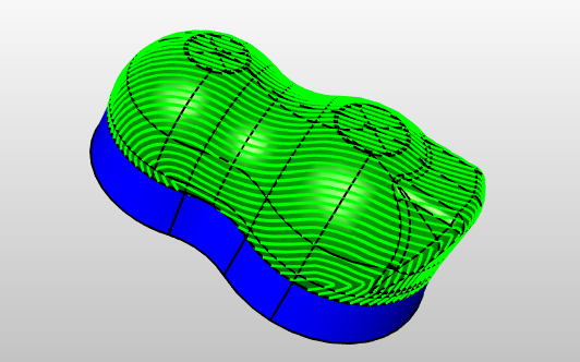
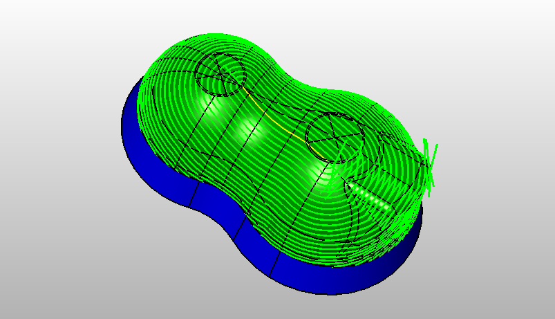
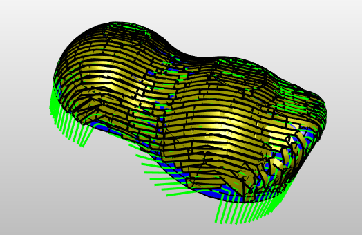
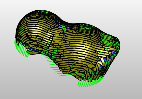
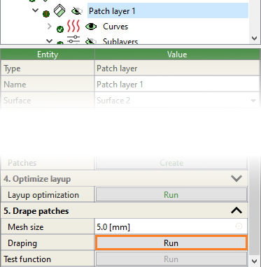
By default, patch creation uses a projection algorithm to approximate the shape of the patches.
This approach is usually sufficient for laminates with slight out-of-plane curvature, as well as
for all laminates with low requirements on the accuracy of the patch preview.
As an additional step, users may drape patches, which results in a more accurate prediction,
especially when working with challenging geometries.
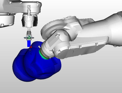
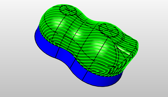
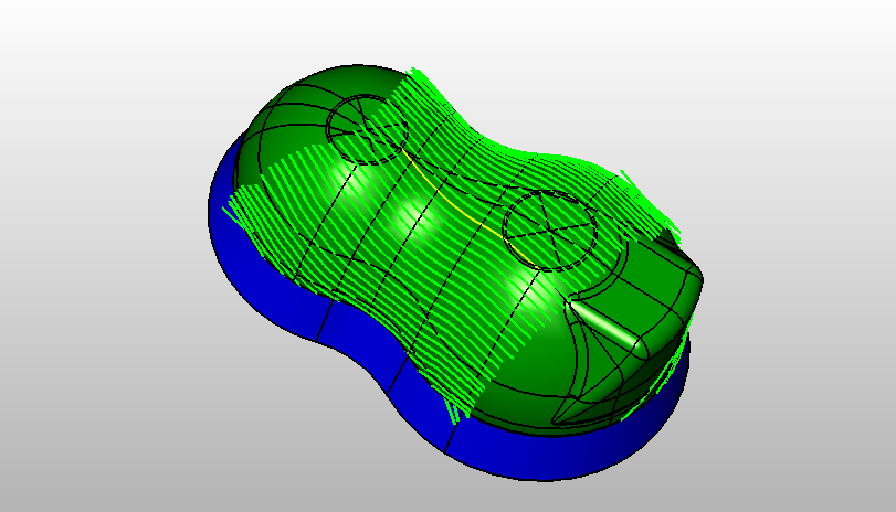
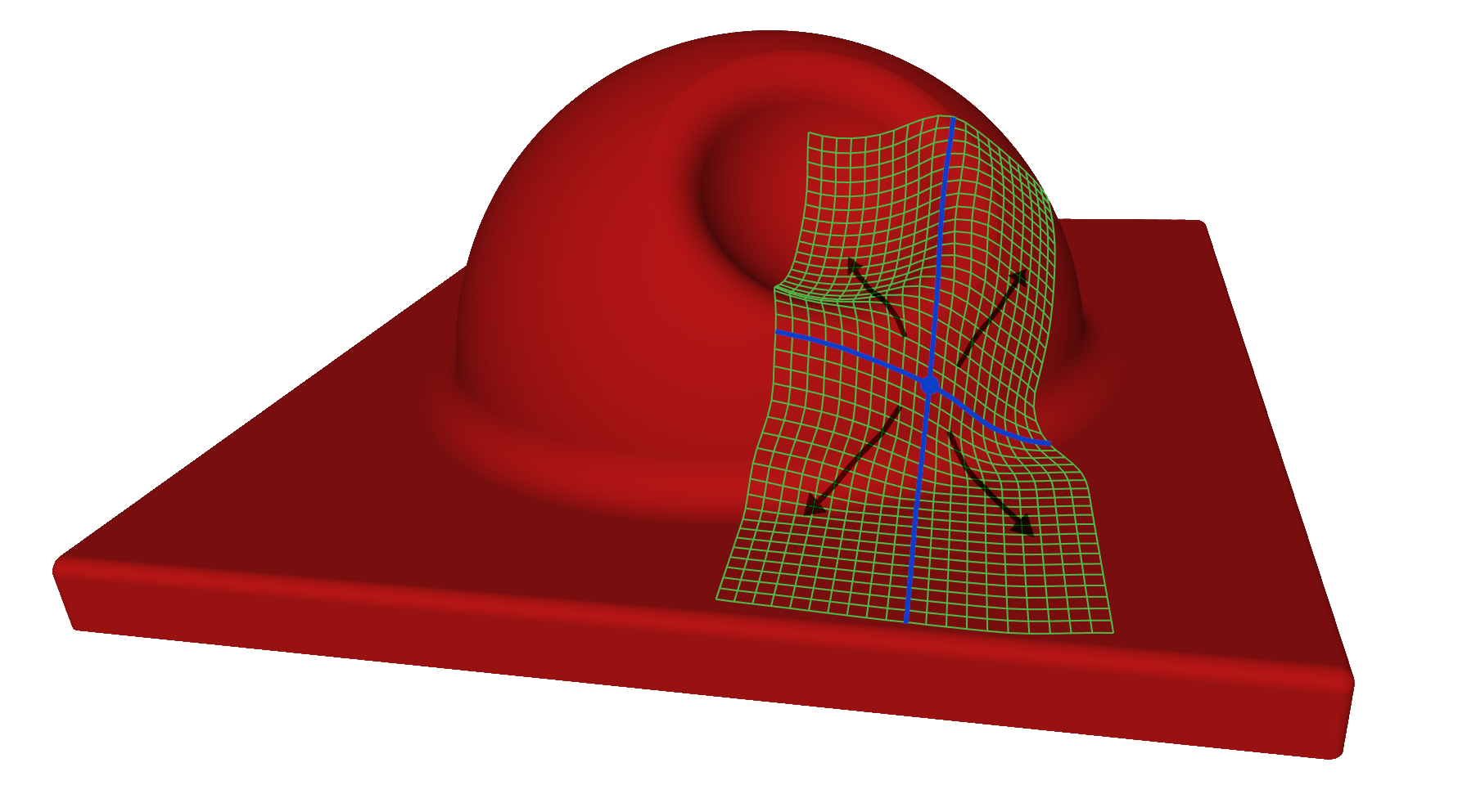
For so called kinematic draping, the center point of each patch and its respective orientation is used to create
two lines on the surface: one in patch direction and the second perpendicular to the first (the blue lines in the image below).
Starting from these two orthogonal lines a mesh with equidistant segment length is propagated
to the corners of the patch. Each node of the patch lies exactly on the surface.
As a consequence, draped patches will look different than their projected counterparts but
their center point will always stay the same. The accuracy of the draping process is
determined by the mesh discretization.
Warning
You should be aware that, although draping is more accurate than projection, it doesn’t take
into account any non-geometric effects like material stiffness, slippage of the patch on the tool surface
or the deformation of the gripper. All of which can cause a significant deviation from the draped geometry.
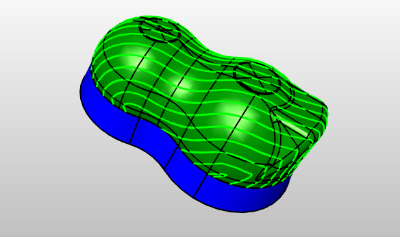
There are three reasons to perform draping on curved geometries:
It improves the prediction of the patch boundary, making it possible to judge very small gaps and overlaps between patches.
It creates a smoother representation of the patch, providing higher preview quality for product visualization.
You can manually move patches (see Manually adjusting positions of patches), change gripper push-in orientation for every patch, or add
additional gripper rolling or separate placement contact points for patches on curved edges (see Gripper handling).
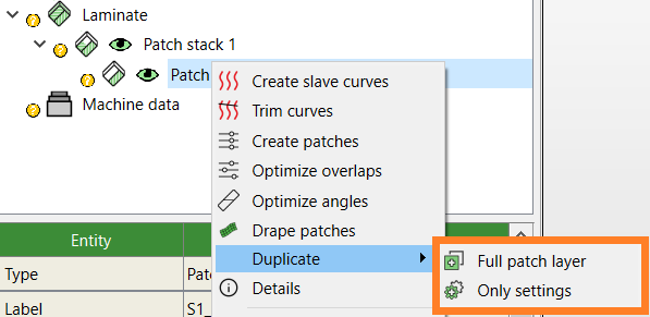
To streamline laminate creation, patch layers can be duplicated. There are two duplication options:
Full patch layer
This will copy the entire patch layer, including all sublayers, chains, and patches.
Only settings
This option duplicates only the settings used for the creation of the slave curves and patches.
Note
If Thick laminates are enabled, excessive use of fully duplicated patch layers might result in inaccuracies in the resultant laminate. This is because thickness offsets are not considered for the duplicated layers.
From here, we need to begin the manufacturing cell simulation. The layup generated by Patch Artist will be available directly in the Motion Artist module so that we can perform the automatic offline programming of the robots. Click on the Motion Artist tab from the green ribbon bar to begin with the robot simulation.
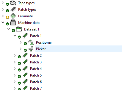
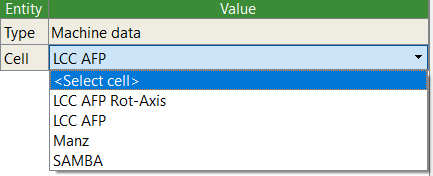
To simulate the manufacturing, the first step after creating the laminate is to create Machine data that can be fed into the manufacturing cell. Machine data basically contains data of robot movements. Artist Studio converts the layup selected by the user into Machine data which the manufacturing cell understands.
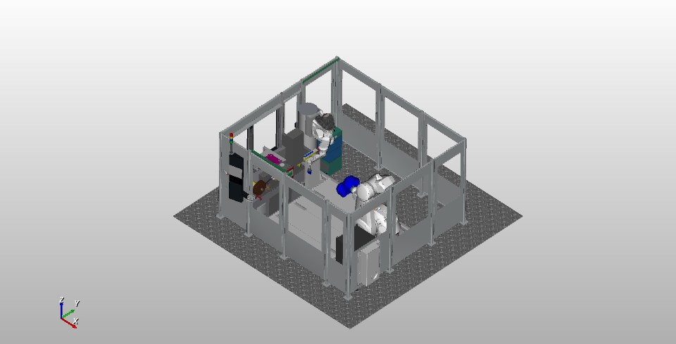
The first step to start with the simulation is to load the manufacturing cell. The manufacturing cell can be selected in the property window after selecting the Machine Data item in the Model Tree.
Click on the drop-down menu under Robot entry and select the cell you wish to load. right click on Machinedata and then click on Loadcell. Then select the manufacturing cell as shown below:
Note
The available manufacturing cells depend on the used module
The appropriate cell geometry will be loaded and shown in the viewport.
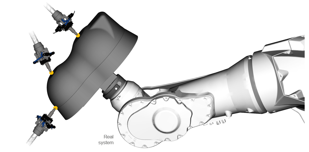
Mount point calibration is the most precise way to define the tool’s coordinate system.
The procedure involves using a physical probing device in place of the patch gripper to collect reference points on the actual tool and then mapping them to the CAD model.
This is an automatic way of calculating the mount point at which the CAD model should be mounted.
Fig. 6.5 Probing multiple points on the tool surface of the real system.
Note
Calculatemountpoint is only recommended to be used with SAMBA PV machines or with SAMBA Pro machines with a Stäubli TX200 positioner
and Stäubli TP80 or TX2-90L picker.
Prepare a notepad or form to note down both positioner joints and picker position for multiple points on the tool.
We recommend to store this data in a spreadsheet.
The position data will be entered into the Calculatemountpoint dialog after the gathering all the necessary data
with the machine.
Before starting to work with the machine, the following should be prepared:
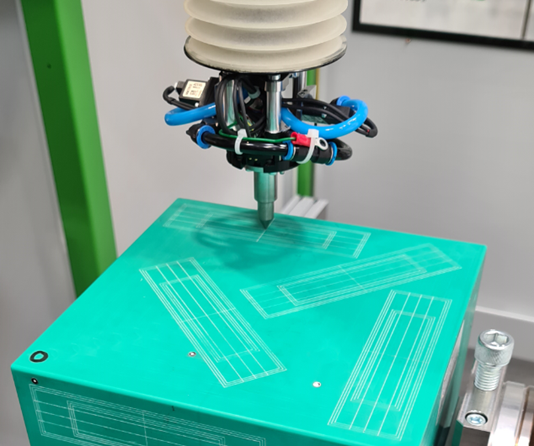
Picker calibration gripper (calibration spike):
Definition of at least 3 different points on the tool that are
Accessible with the picker calibration gripper
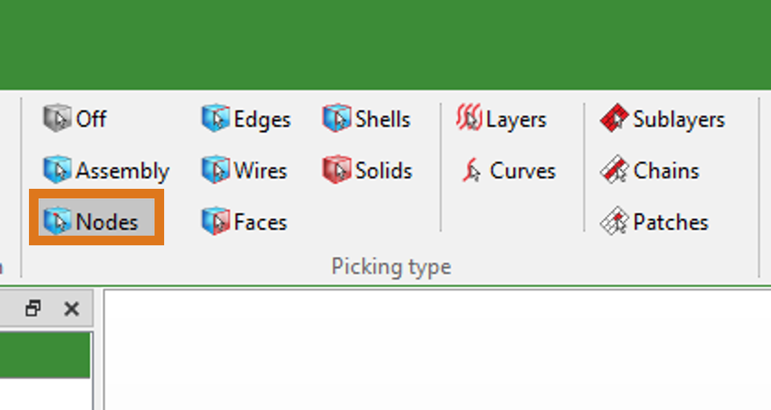
Pickable with Nodes Picking type in Artist Studio
Afterwards, the machine itself can be prepared for gathering the data by following these steps:
Mount the preforming tool to the positioner.
Remove the patch gripper and replace it with the picker calibration gripper.
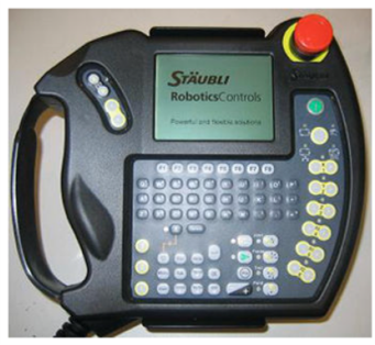
Connect the teach pendant to the positioner (Stäubli TX200)
After the preparations, start by first moving the positioner:
Move positioner with tool into a position that allows accessing the point on the tool with the calibration spike
Let go of dead man’s switch on teach pendant
→ TX200 will apply its breaks and hold its position
Note down which point on the tool is to be probed
Press button on the teach pendant
Navigate to Control Panel (Systemsteuerung) and select by pressing return button:
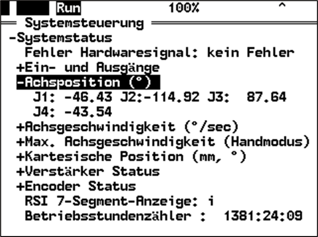
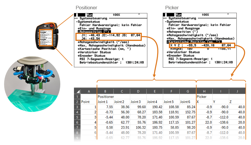
Expand Controller status (Systemstatus) and then the sub-item Axis position (°) (Achsposition (°)):
Example view of Achsposition (°)
Note down the joint values J1 - J6 for the TX200
Move picker
Then, continue with the picker:
Warning
For machines with the Stäubli TP80 picker robot, the dead man’s switch has to kept on until after
noting down the position values. This is to prevent the robot from moving slightly after turning of the drives.
This will reduce the accuracy of the picked point.
Other picker robot types, e.g. Stäubli TX2-90L or KUKA 6-axis robots, are unaffected by this potential issue
and will apply their breaks.
Connect the teach pendant to the TP80 or switch to the teach pendant of the TP80 / TX2-90L
With the teach pendant and the mounted calibration spike, jog the picker to probe the position on the tool.
Press button on teach pendant to open the menu
Navigate to Control Panel (Systemsteuerung) and select by pressing return button:
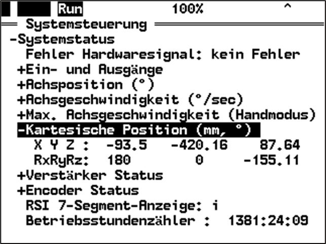
Expand Controller status (Systemstatus) and then the sub-item Cartesian position (mm, °) (Kartesische position (mm, °)):
Example view of Kartesische Position (mm, °)
Note down the X, Y, and Z values. Rx, Ry, and Rz are not used and do not need to be noted down.
This process will have to be repeated to end up with at least three sets of values of positioner joints
and picker cartesian position for each probed point.
Fig. 6.6 Robot joint positions and coordinates stored in a spreadsheet during the probing process.
Note
If multiple points can be measured with the same tool position, i.e. the positioner does not need to be moved,
it is valid to reuse the same positioner stance and joint values.
Note
The same point can be probed multiple times but this will not lift the requirement to probe three different points on the tool.
Note
There is no limit on the number of probed points on the tool. Three points already result in accurate positioning but it can be
beneficial to probe four or five points to further reduce the measurement error.
After gathering the data, continue with the next section to run the Mount point calculation in Artist Studio.
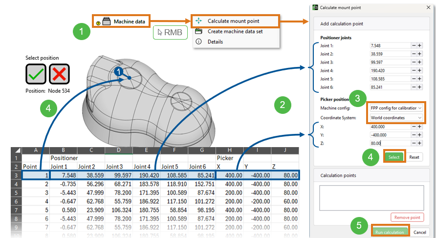
To calculate the mount point from the gathered data, follow these steps:
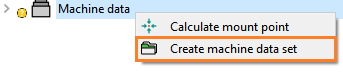
Right click on Machinedata and select Calculatemountpoint.
Enter the values of Positioner joints and Picker position for a point in the Calculatemountpoint dialog box.
Under the option CoordinateSystem, select an appropriate coordinate system for your robotic tool.
The default for the SAMBA Pro and the SAMBA PV system is Worldcoordinates while other systems like the Manz FPP cell require selecting Robotcoordinates.
Fig. 6.7 Running the mount point calculation in ARTIST STUDIO.
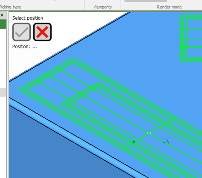
Now click on the Select button to select points from the imported geometry.
The previous action will take you to Patch Artist and allows selecting a point on the geometry. After selecting the probed point on the geometry, click on .
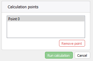
The selected point will be added with the joint and position data to the list of calculation points.
Repeat steps 2 to 5 until having entered all point data.
In case of incorrectly entered values, these can be removed with the Remove button.
The Runcalculation button will turn active once at least three different points have been added.
Click on Runcalculation to calculate the mount point.
Artist Studio will calculate the optimal transformation of the tool as your new mount point.
It will be created as a new system in the CAD model and selected as your current mount point.
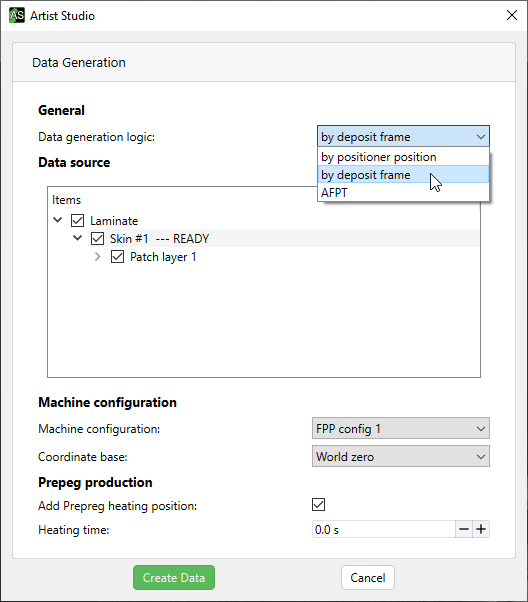
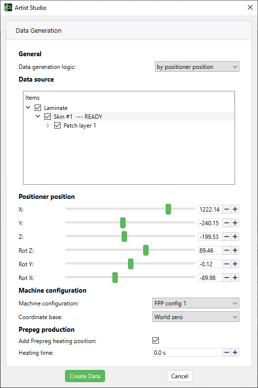
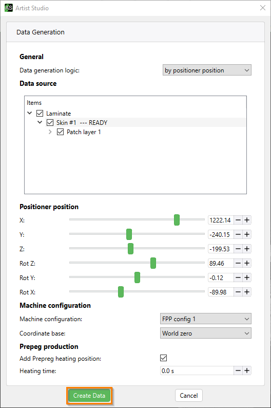
A DataGeneration window will appear in which the user can select and specify the data generation logic for the data set. Depending on the type of model the user can select ‘by positioner position’ or ‘by deposit frame’.
Data generation logic: by positioner position
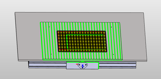
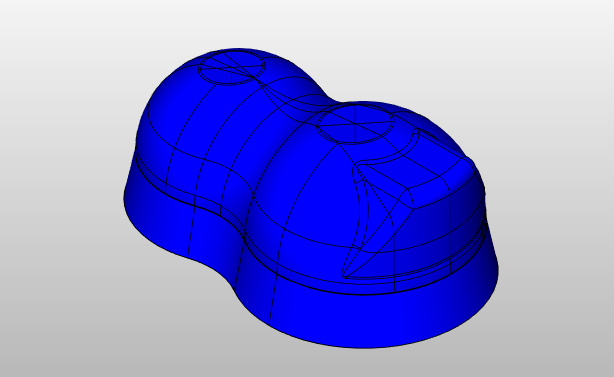
This mode can be used when it is desirable to move the tool as little as possible (example use case shown in the figure below). Here, only the Picker robot will make movements in order to patch the surface and the Positioner robot will hold the tool at a fixed position.
Data source
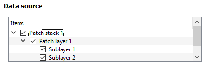
Datasource is a common setting available for all types of data generation logic. It allows the user to select
or deselect any stack, layer, or sublayer to define which parts of the model will be used for creating a dataset.
Starting with production systems released in 2024 and later, multiple patch lengths are supported within a single robot program.
This allows you to:
Select multiple layers with different patch types
Include layers where individual patches have manually overridden patch types
After the data set has been generated, you can use the Details popup to view the number of patches of each shape.
Note
Production systems older than 2024 support only one patch length per robot program.
For these systems, ensure that all selected (sub)layers use patches of only one patch type.
Note
For systems with one spool of material (one cutting belt), you cannot combine different patch widths in a single robot program.
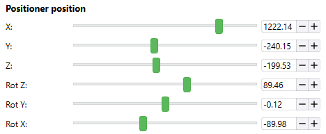
Positioner position
The position at which the Positioner robot will hold the tool is defined here. This position will be fixed for a particular data set.
During patching, the Picker robot will make the necessary movements and the position of the Positioner robot will remain fixed.
Data generation logic: by deposit frame
Bydepositframe mode can be used when the model is 3-Dimensional and curvy in nature as shown in the figure below. The model will be attached directly to the Positioner robot. The Picker and Positioner robots will make movements simultaneously for the patching of patches on the model’s surface.
Prepreg production
The heating unit in the manufacturing cell provides sufficient heating for the resin of the tape (on the gripper) to heat up so that it can be smoothly patched on the surface of the CAD model. However, some tapes can’t be heated using this heating unit as it might get stick to the gripper. To solve this problem, Prepreg production is required. This process heats the tape externally with the Infrared rays.
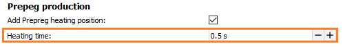
To start Prepreg production check the Addprepregheatingposition button.
Enter the value for Heatingtime for example, 0.5s to define the time for heating.
Create Data
After defining a data type mode and specifying other options of Data generation, the user can fill the dataset with the data by clicking on CreateData button.
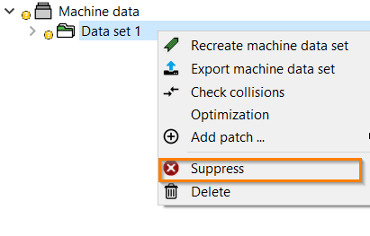
A data set will be created which will contain the data for your simulation. However, if you want to split the laminate layup into several files then different datasets should be created for different files. To do this, right click on the layer you don’t want to be filled in the data set and click on the Suppress option.
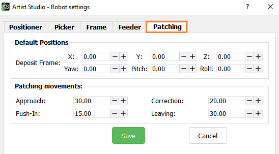
In Motion Artist to simulate the manufacturing cell, the first requirement is to set Deposit Frame where the interaction of robots - Picker and Positioner will occur.
To set Deposit Frame click on the Robot settings option under Miscellaneous group and select the Patching tab.
Enter the appropriate values for X, Y, Z axis and respective Yaw, Pitch and Roll values under the Deposit Frame.
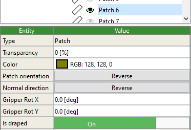
The patches filled in Data set are represented by different colors in front of their patch name. These colored icons show the status of patches in Data set which are explained as:
- This is because of two reasons:
Limit reached - This icon represents that the movement of the robot has reached its limit and cannot move further. As shown below, the fifth axes of Positioner has reached its limit i.e 120.000. This error can be corrected by optimization or by modifying the patch.
Collision - When a collision is detected in robot movements after checking the collision then turns into .
- This means the robot movements are fine but the collision is not yet checked. To correct this check the collision of the patch. If after checking the collision, it turns into then optimize or modify the patch.
- This is known for the force correction of a patch at your own risk. Sometimes, you know that the robot movements will not collide even if it is showing and you want to pass it on for patching. This can be done by by the Override collision option. This overriding of a patch is shown by .
- When a robot movement is smooth without any collision and ready for patching then it is represented by a icon.
Note
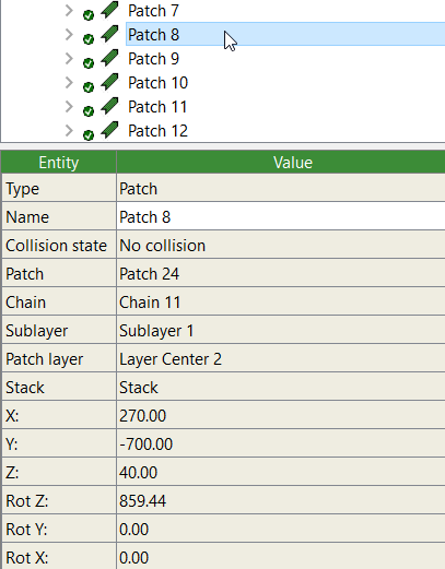
When clicking on a patch in the list, a property window of the selected patch as shown below consisted of various entities such as Type, Name, Collision state and Position will appear.
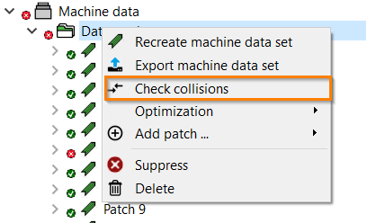
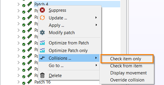
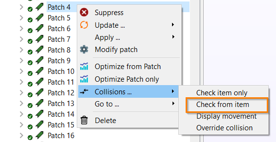
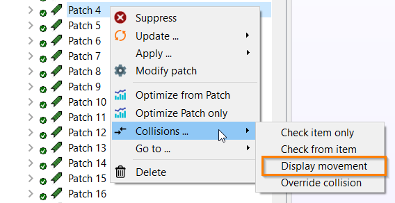
It is important to detect collisions before creating the layup. Collisions can be detected in following ways:
Complete dataset - Select the dataset and click right. Then click on Checkcollisions.
One patch - Click right on the patch and select Collisions. From the Collisions context menu click on Checkitemonly.
From patch - Check from patch means that all the patches starting from the currently selected one will be checked for the collision. To detect collisions from a particular patch follow these steps:
Click right on the patch and select Collisions. From the Collisions context menu click on Checkfromitem.
Patches with collisions will be shown by and with no collisions by .
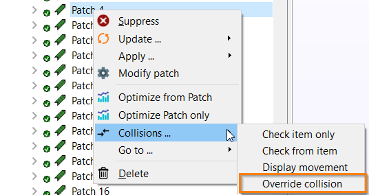
This is a force method to override collisions. Motion Artist is normally using a safety distance of 3 cm to avoid any collision. Override collision is recommended when you are sure enough that collision is not occurring and you want to pass it on for patching. To override collision follow these steps:
Right click on the patch and select Collisions.
Then select Overridecollision from the context menu of Collisions.
The created data set may have errors due to patches having collisions or being unreachable. Artist Studio supports
optimizations that aim to automatically adjust the patch deposit frame to have patches both collision-free and reachable.
The Simple Optimization varies between ‘by positioner position’ and ‘by deposit frame’ data sets. For the latter, it tries to optimize a patch’s
deposit frame by modifying the rotation around the z-axis. In contrast, when used with ‘by positioner position’ data sets, it modifies the
x and y values of the deposit frame instead.
Both approaches have the common goal of achieving a patch position that is:
reachable
collision-free
leads to minimal movement time from previous patch for positioner
There are three ways to optimize the patches:
Complete dataset - To optimize the complete dataset, right click on the created data set and select Optimizemovements under the option Optimization to optimize all the patches in a particular dataset.
One patch - For optimization of a specific patch, right click on the selected patch and click on Optimizepatchonly.
From patch - To optimize all the patches starting from a specific patch, right click on the selected patch and click on Optimizefrompatch.
It is also possible to use Optimizepatchonly while having multiple patches selected.
Deposit optimization has been introduced in version 1.3.23. However, it is still under active development and might
end up with unexpected results or cause other related issues while optimizing a dataset. Please ensure necessary
precautions are taken, e.g. save a version of the file before running the deposit optimization.
The deposit optimization has been specifically developed for a version of SAMBA PRO that is using two 6-axis robots.
As a result of that, the deposit frame is no longer bound to be pointing upwards.
In order to put this flexibility to good use, this type of optimization supports optimizing the deposit frame with up
to 6 degrees of freedom.
The type of production system used will decide whether the reachability optimization or the deposit optimization
dialog will be displayed. Currently, deposit optimization is only supported for 12-axis production systems.
The deposit optimization dialog allows setting the optimization type. Currently, only the COBYLA algorithm is supported.
In addition to that, both the optimization constraints and the stopping criteria can be adjusted to one’s needs:
Maximum iterations:
Specifies how many iterations should be run before stopping/aborting the optimization
Initial step size:
Defines the percentage to use for calculating the default step size value. A value of 50% results in the initial
step size being 50% of the optimization bandwidth, i.e. 50% of the absolute difference between the maximum and
minimum value of each coordinate.
A minimum value of 200 and maximum value of 600 will result in an initial step size of 200 when this setting is
set to 50%.
Min / max coordinate values:
Specify the minimum and maximum values to use for each coordinate. Setting the minimum and maximum value to the
same value will result in this value being fixed.
Absolute parameter tolerance:
Optimization will stop when change of coordinates is below this value, i.e. the current step size is smaller
than this value for any given coordinate (except for ones with fixed values): \({\Delta} x\)
Relative parameter tolerance:
Optimization will stop when the gradient between two consecutive values is below the specified value:
\({\Delta} x / x_i\)
Absolute quality tolerance:
Optimization will stop when change of calculated “quality” of a patch is below this value:
\({\Delta} f\)
Relative quality tolerance:
Optimization will stop when gradient between two consecutive quality values is below specified value:
\({\Delta} f / f_i\)
Stop value:
Value that is deemed a “good solution”. The default value of 10 will result in the optimization using any deposit frame
that is both reachable and collision free. It will not optimize the position for the quickest placement.
Deposit frames with a collision are penalized with a value of 1000, unreachable ones with a value of 2000.
As a result of that, the optimization will prefer positions with collisions (which are easier to be adjusted manually)
over unreachable ones.
The optimization can be run by clicking on Start optimization and will require some time to run. During each
iteration, the patch positions are calculated and collisions are checked. In addition to the starting deposit frame,
runtime of this optimization highly depends on the complexity and size of the part to produce and the cell itself.
Collision avoidance can be used to prevent or reduce the risk of collisions during
movements of the Picker between the camera and placement position of a patch. It allows users
to manually add additional avoidance points before the Approach and after the Leaving positions
of the patch placement. These can then be applied to the complete dataset from the model explorer.
While multiple avoidance points can be added, the maximum number of avoidance points can be limited
depending on the machine used. By default, at least two avoidance points before the patch placement
and two after the patch placement, i.e. two avoidance points added via menu, are supported on all
shipped machines.
Note
The Collision avoidance feature was first introduced in Artist Studio 1.3.36
Before setting the desired robot position, expand the tree of the patch of the data set to
which you want to add avoidance points:
Also ensure that you are currently using Motion Artist or switch to the Motion Artist tab.
To add an avoidance point, follow these steps:
Adjust the axis values of the picker in the Ribbon bar
Right-click on Picker and choose Add...>Avoidancepoint
Wait until avoidance point is added to the patch.
Note
While adding the point, Motion Artist will check the patch for collisions.
This can take some time to be processed.
As a result, in fact two avoidance movements will be added:
Every time you add an avoidance point, this extra position will be used by the Picker while moving
from the camera to the approach position and while moving back from the leaving position
to the camera.
Avoidance points can be added manually to any data-set patches. However, the avoidance points
added to the first patch are special: they can be applied to the rest of the data set.
Warning
Any avoidance points that were added to any patch other than the first patch will be
overwritten while applying the avoidance points.
To apply the avoidance point(s) of the first patch to the rest of the data set, follow these steps:
Right-click on the data set
Click on Apply...>Avoidancetodataset
Wait until avoidance points have been added to the data set
Note
After applying the avoidance points to the data set, Motion Artist will automatically
check the complete data set for collisions. This process might take a long time depending on
the amount of patches in your data set.
Hint
There is no need to remove the avoidance points from all patches before applying avoidance
points to the data set again. While applying the avoidance points from the first patch,
Motion Artist will automatically remove first any old avoidance points.
You can manually remove avoidance points one by one. This might make sense in some cases where this
extra position is only needed while moving to the preforming tool or back from it.
This can be done by right-clicking on the Avoidance Point movement you want to delete and selecting
Delete from the context menu.
It’s also possible to remove all avoidance points from the data set:
Delete all avoidance points from the first patch of the data set
Apply avoidance points (from the first patch) to the data set
As a result, all avoidance points will be deleted.
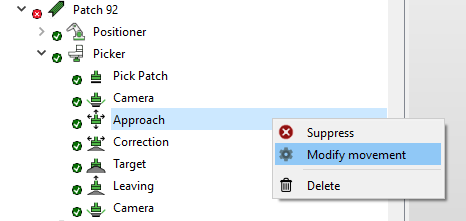
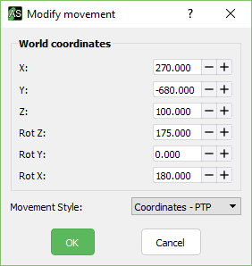
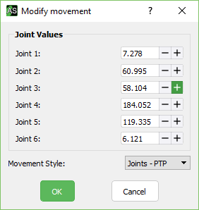
A dialog will be opened which will allow you to change the coordinate or joint values, depending on which type of robot is used.
The Movementstyle setting will allow you to also adjust the type of movement that will be executed by the robot.
Depending on the robot used, some of these movement types will be available:
Coordinates - Linear
Coordinates - PTP
Joints - Linear
Joints - PTP
Note
Depending on the used manufacturing cell, some of the movement styles might not be supported.
Consult the machine documentation if unsure.
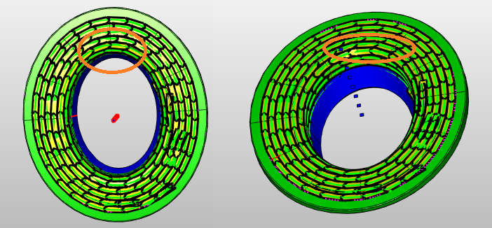
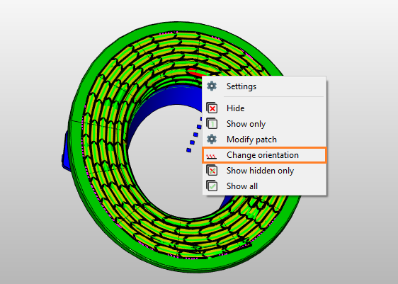
The orientation of normals of the patches is responsible for the direction of Picker robot with which it will patch on the surface of a geometry. However, the robot may not be able to patch on curvy surfaces.
For patching on curvy surfaces you need to change the orientation of the normals. To change the orientation follow these steps:
Select the patch name from the dataset for whom you want to change the orientation.
Go to Patch Artist and click on Patches from the Ribbon bar under Pickingtype group.
The selected patch will be highlighted(red) in the viewport. To view the orientation of normal select Showorientation from the Ribbon bar under Rendermode group.
Right click on the patch and select Changeorientation.
This will open a pop-up. Here, you can change the orientation of the normal.

 - Select one face and click on this icon. With every click, adjacent faces will be selected.
 - Select one face of the assembly and then click on this icon. It will select the whole assembly corresponding to the selected face.
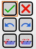
 - Select one edge and click on this icon. With every click, the adjacent edges will be selected.
 - Select one edge of the assembly and click on this icon. It will select the whole assembly corresponding to the selected surface.


 button on the teach pendant
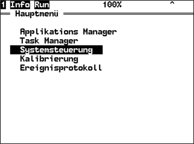
 .
.
 - This is because of two reasons:
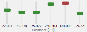
 turns into
  - This is known for the force correction of a patch at your own risk. Sometimes, you know that the robot movements will not collide even if it is showing
  - When a robot movement is smooth without any collision and ready for patching then it is represented by a